Simple Linear Regression

Machine Learning → Supervised Learning → Regression → Linear Regression

Simple Linear Regression (SLR) is a fundamental algorithm in statistics and machine learning. It is used to model the relationship between two variables: one independent (input) and one dependent (output). It is ideal for situations where we want to determine if and how these two variables are related. It is commonly used for predicting values, estimating trends, and clarifying relationships in data. SLR belongs to the broader field of data analysis known as regression analysis.

Although it is a very simple model, it serves as a foundational building block for understanding more complex techniques such as multiple linear regression, decision trees, or neural networks.

How It Works

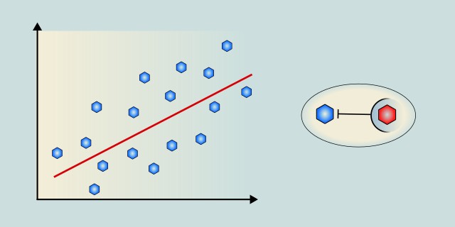
Simple Linear Regression seeks the simplest possible relationship between two variables, a straight line that best fits the data points in a graph.

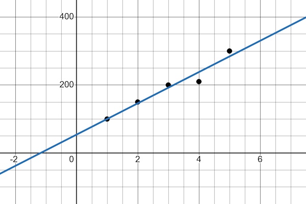
Imagine we want to find out whether the amount of coffee a programmer drinks during the day affects the number of lines of code they write. Suppose we have a table of such data. One column contains the number of cups of coffee consumed, and the other shows the number of lines of code written. If we plot these pairs of values on a graph, we’ll get a scattered “cloud” of points.

You can plot these value pairs on a graph:

X-axis (horizontal) – number of cups of coffee
Y-axis (vertical) – number of lines of code

The task of linear regression is to find a line that best fits these points.

Process

In practice, we could proceed as follows:

First, we collect historical data, in our case, the number of coffee cups consumed and how many lines of code the programmer wrote afterward. Then, we find the equation, or more precisely, calculate the best-fitting line that describes the trend in our data. Once we know the equation of this line, we can estimate the outcome even for values we haven’t observed yet.

This approach is used whenever there is a reasonable assumption that a linear relationship exists between two variables.

Mathematical Foundation

Simple Linear Regression looks for the simplest relationship between two variables: a straight line that best describes their connection. This relationship is expressed using a linear equation:

$$ y = b_1 \cdot x + b_0 $$

$x$ – independent variable (e.g., cups of coffee)
$y$ – dependent variable (e.g., lines of code)
$b_1$ – slope (how much y changes when x increases by 1)
$b_0$ – y-intercept (value of y when x = 0)

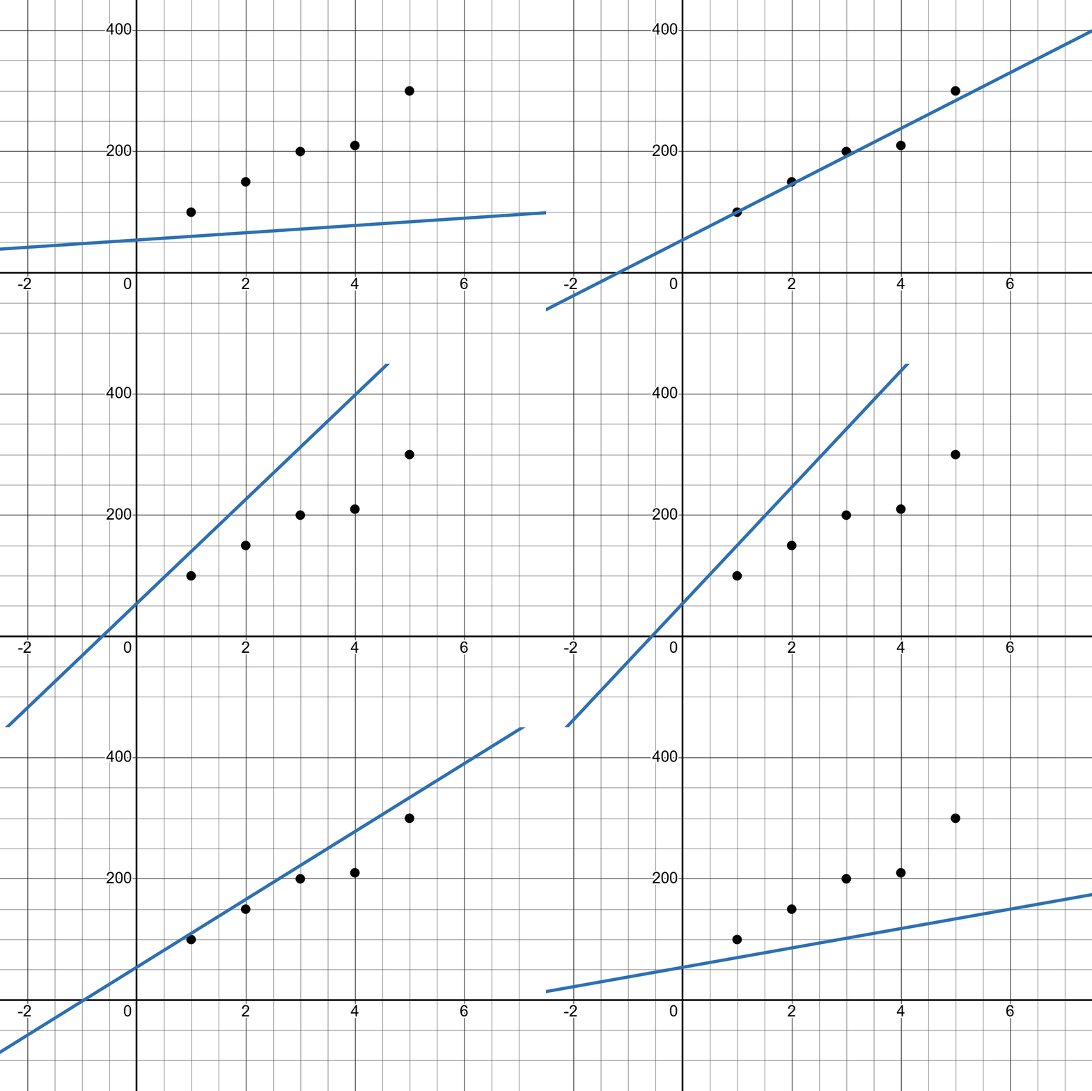
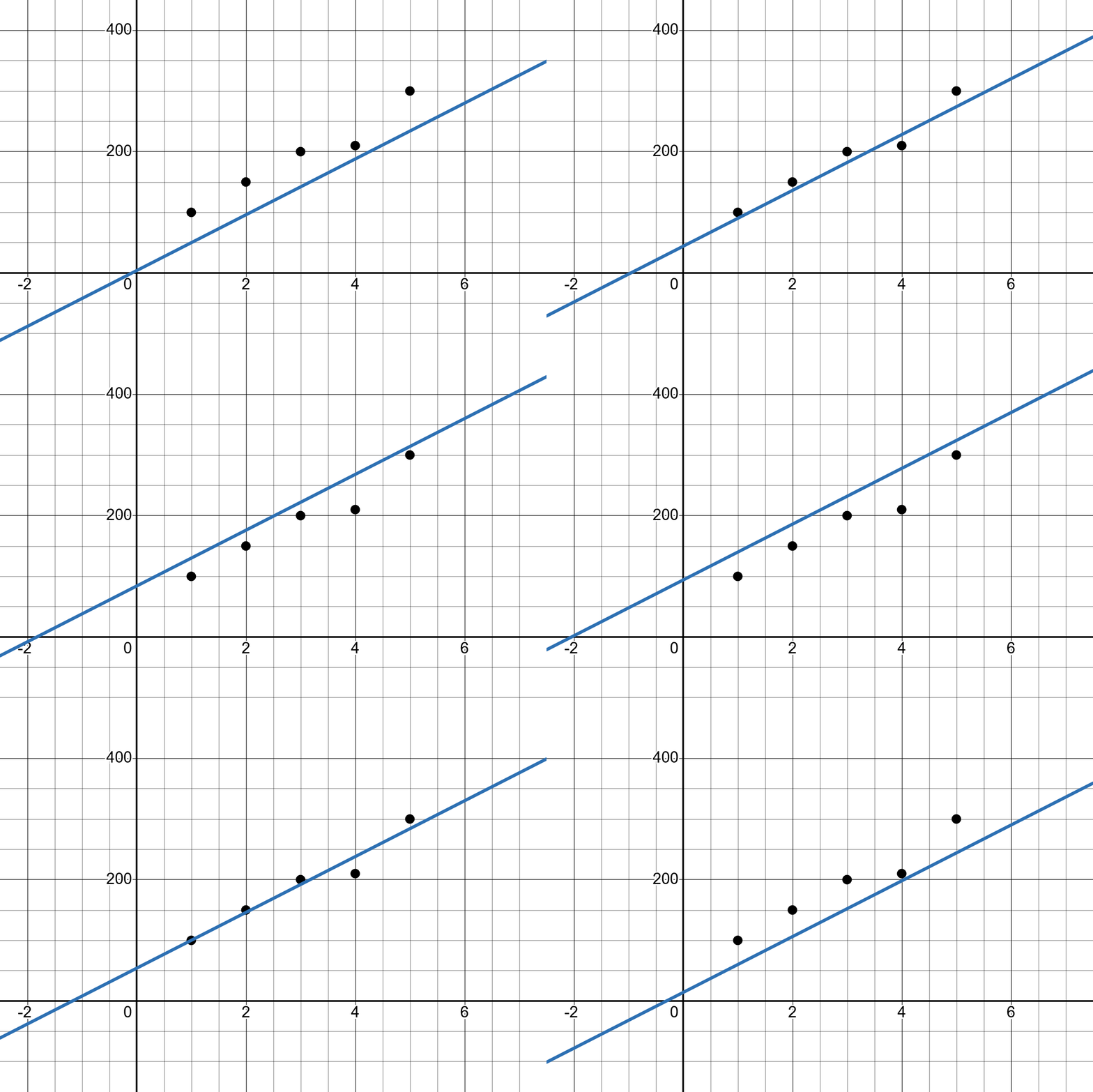
Finding this line means determining the values of $b_1$ and $b_0$ such that the prediction error is as small as possible. The error is the difference between the actual value and the value predicted by the line.

There are several ways to compute this line. The result is fully determined by two parameters: the y-intercept and the slope. These define how the final line will look.

Slope: The slope of the line $b_1$ indicates how much the value of $y$ changes when $x$ increases by one unit.

Intercept: The intercept $b_0$ represents the point where the regression line crosses the y-axis.

Direct Analytical Solution (Least Squares Method)

This approach uses a statistical formula to directly compute the values of the parameters $b_0$ and $b_1$. Here, $b_1$ is the slope of the line that best fits the known data points, and $b_0$ is the intercept of that line with the y-axis.

The slope and intercept are calculated using the following formulas:

Slope:$$ b_1 = \frac{ \sum (x_i - \bar{x})(y_i - \bar{y}) }{ \sum (x_i - \bar{x})^2 } $$Intercept:$$ b_0 = \bar{y} - b_1 \cdot \bar{x} $$

$\bar{x}$ – is the mean of the input (independent) variable.
$\bar{y}$ – is the mean of the output (dependent) variable.

Iterative Optimization Using Algorithms (e.g., Gradient Descent)

Gradient Descent is an algorithm that repeatedly adjusts the parameters in order to minimize the prediction error. It is an alternative to the direct analytical solution, especially useful when working with large datasets. Although it is not commonly used for solving simple linear regression problems, it becomes relevant in cases like Multiple Linear Regression or when the dataset is too large to optimize analytically or to reduce manually.

Note: The result of both methods is a simple model that can estimate (predict) the value of $y$ based on a known value of $x$. We plug the calculated intercept $b_0$, the slope $b_1$, and the known input $x$ (e.g., number of coffee cups) into the equation above. This allows us to predict how many lines of code ($y$) a programmer will write after drinking $x$ cups of coffee.

Code Example: Programmer performance

This example demonstrates how to implement Simple Linear Regression in Rust using the least squares method. The function simple_linear_regression calculates the slope and intercept of the regression line based on the given data. It models the relationship between the number of coffee cups a programmer drinks (x) and the number of lines of code they write (y). Written in Rust.

// It calculates the slope (m) and intercept (b) of the best fit line using the least squares method.
fn simple_linear_regression(x: &[f64], y: &[f64]) -> (f64, f64) {
    assert_eq!(x.len(), y.len(), "The lengths of the inputs do not match");
    let n = x.len() as f64;

    // Calculate the sums: Σx, Σy, Σ(xy), Σ(x^2)
    let sum_x = x.iter().sum::<f64>();
    let sum_y = y.iter().sum::<f64>();
    let sum_xy = x.iter().zip(y.iter()).map(|(xi, yi)| xi * yi).sum::<f64>();
    let sum_x2 = x.iter().map(|xi| xi * xi).sum::<f64>();

    // Calculateslope: m = (n * Σ(xy) - Σx * Σy) / (n * Σ(x^2) - (Σx)^2)
    let m = (n * sum_xy - sum_x * sum_y) / (n * sum_x2 - sum_x * sum_x);

    // Calculate intercept: b = (Σy - m * Σx) / n
    let b = (sum_y - m * sum_x) / n;

    (m, b)
}

// Function to predict y given x, slope (m), and intercept (b)
fn predict(x: f64, m: f64, b: f64) -> f64 {
    m * x + b
}

fn main() {
    // Example data points for linear regression
    // x: independent variable, y: dependent variable
    let x = [1.0, 2.0, 3.0, 4.0, 5.0];
    let y = [100.0, 150.0, 200.0, 210.0, 300.0];

    // Perform linear regression to find the slope and intercept
    let (m, b) = simple_linear_regression(&x, &y);

    // Output the model parameters
    println!("Model: y = {:.4}x + {:.4}", m, b);

    // Predict a value for a new input
    // For example, predict y for x = 8.0
    let test_x = 8.0;
    let predicted = predict(test_x, m, b);

    println!("For x = {:.1}, predicted y = {:.3}", test_x, predicted);
}

Model Evaluation – Prediction Error

It is always important to verify how accurate our model is. This helps determine whether linear regression is even appropriate. If the error is large, the relationship might be nonlinear, or the data may be too scattered. It can also help identify problematic data points or outliers.

To evaluate the model, we use various error metrics that quantify the difference between the actual values and the model’s predictions:

Residual

A residual tells us how much a specific prediction deviated from the actual result.

It is the difference between the true value and the predicted value:

$$ \varepsilon_i = y_i - \hat{y}_i $$

👉 A detailed explanation of residuals can be found in the section: Residuals

MSE (Mean Squared Error)

MSE penalizes larger errors more than smaller ones (because the error is squared).

It represents the average squared difference between the actual and predicted values:

$$ \text{MSE} = \frac{1}{n} \sum_{i=1}^{n} (y_i - \hat{y}_i)^2 $$

👉 A detailed explanation of MSE can be found in the section: Mean Squared Error

RMSE (Root Mean Squared Error)

RMSE has the same units as the original values, making it more intuitive to interpret.

It represents the average squared difference between the actual and predicted values:

$$ \text{RMSE} = \sqrt{\text{MSE}} $$

👉 A detailed explanation of RMSE can be found in the section: Root Mean Squared Error

R² (Coefficient of Determination)

R² indicates how much of the variability in the data can be explained by the model:

$$ R^2 = 1 - \frac{\sum (y_i - \hat{y}_i)^2}{\sum (y_i - \bar{y})^2} $$

Close to 1 – the model explains the variability in the data very well.
Close to 0 – the model explains very little of the variability.

👉 A detailed explanation of R² can be found in the section: R² Coefficient of Determination

Alternative Algorithms

While Simple Linear Regression is effective for modeling the relationship between two variables, there are often more suitable or powerful alternatives. These are especially useful when the relationship is non-linear, when working with more than two variables, when the data contains noise, or when a more robust and flexible model is required.

Multiple Linear Regression: Models the relationship between two or more independent variables and a dependent variable. Learn more
Decision Tree Regression: Uses tree-based models for regression tasks. Learn more
Support Vector Regression: Uses support vector machines for regression. Learn more

Advantages and Disadvantages

✅ Advantages:

Simple to implement.
Produces results that are easy to interpret.
Fast computation.
Serves as a solid foundation for more complex models.

❌ Disadvantages:

Only works well when the relationship is linear.
Not suitable for complex tasks.
Sensitive to extreme values (outliers).
Assumes errors are normally distributed with constant variance (homoscedasticity).

Quick Recommendations

Criterion	Recommendation
Dataset Size	🟢 Small / 🟡 Medium
Training Complexity	🟢 Low

Use Case Examples

House Price Prediction

Estimating house prices based on size or location. This involves modeling how the price changes as the square footage or the neighborhood changes, helping buyers and sellers understand market trends.

Salary Estimation

Predicting salary based on years of experience. Simple Linear Regression can highlight how increases in professional experience tend to correlate with salary growth, providing insights for career planning.

Advertising Impact

Analyzing sales changes relative to advertising spend. This helps businesses evaluate how much additional revenue is generated per dollar invested in advertising campaigns.

Exam Score Prediction

Forecasting exam results based on hours studied. It allows students and educators to understand the likely impact of study time on academic performance.

GDP Growth Forecast

Predicting GDP growth from historical economic indicators. By examining a single influential factor such as export volume or investment, this helps economists anticipate future economic trends.

Conclusion

Simple Linear Regression is a fundamental building block in both machine learning and statistics. Although it is a simple technique, it serves as an excellent tool for explaining relationships between two variables and forms the foundation for understanding more complex models, such as multiple linear regression or neural networks.

External resources:

Example code in Rust available on 👉 GitHub Repository

Feedback

Found this helpful? Let me know what you think or suggest improvements 👉 Contact me.